ONLINE EXTRA: Using GPS Velocity Vectors to Illustrate Elastic Rebound

MICHAEL R. BRUDZINSKI is a professor in the Department of Geology and Environmental Earth Sciences at Miami University, Oxford, OH

Introduction

Many of the different models for elastic rebound described in this issue are driven by the difficulty in creating a visualization of the actual process that operates on faults. Rock near a fault are bent on the order of a few meters relative to rocks far from the fault, but this bending can occur over tens of kilometers of distance. The gradual bending near active faults can build up over tens to hundreds of years, but when an earthquake occurs, the rocks move in matter of seconds. Students typically see only the results of an earthquake, such as the offset of a fence built across a fault (Figure 1a), but not the gradual motion that precedes an earthquake. Students may learn how to characterize faults based on their offset (Figure 1b), but have a harder time learning what leads to those offsets.

Fortunately for geoscientists, the increasing precision of instruments enables them to measure gradual motions along faults in great detail. One of the most common strategies is to attach a high precision GPS receiver to a rock exposure and then record its daily position over many years using satellites. When a network of these GPS stations are installed around a fault, the process of rock bending can be observed in the variations of ground motion from near the fault to far away. This article describes efforts to utilize patterns of GPS data to help students visualize the elastic rebound concept.

Assignment

Students are initially introduced to elastic rebound theory via a lecture about the 1906 San Francisco earthquake, including much of the information described in the article by Dolphin in this issue on the history of elastic rebound theory. The lecture includes animations to help students visualize the alternating phases of gradual rock bending over long time frames and rapid fault motion over seconds. IRIS provides animations with accompanying explanations that help illustrate these concepts. (http://www.iris.edu/hq/inclass/animation/elastic_rebound_on_highfriction_strikeslip_fault). The pre-assignment lecture also introduces students to the concept of geodesy, where scientists measure changes in the Earth's surface over time with things like precise GPS instruments.

Students are then given a map view diagram (i.e., top down view; Figure 2) of a fence that is built across a right-lateral strike-slip fault, similar to the real situation shown in Figure 1. The map is designed to illustrate simple fault motion and the small arrows on either side of the fault indicate one side is moving in the opposite direction than the other side of the fault. Given the diagram shown in Figure 2a, the students are asked to predict (by either choosing or sketching) the expected pattern of how the fence will change shape at three points of time in the future: 100 years after the fence was built, but prior to an earthquake (Figure 2b): immediately after an earthquake (Figure 2c): and 100 years after an earthquake (Figure 2d). Answering these questions helps students consider how rocks bend near a fault as a key part of elastic rebound. Additional help for the students comes from "worked examples," in which students are progressively told which answers are wrong and consider reasons why, followed by which answers are right. (This strategy arose through collaborative work in the GET-Spatial Learning Network: https://serc.carleton.edu/getspatial).

Figure 3 shows the same situations as Figure 2, but using GPS velocity arrows instead of a fence to illustrate motion. Students are given a map view of the same right-lateral strike-slip fault and are asked to draw the velocities expected at each GPS site for before, during, and after an earthquake. Before the earthquake, the fault is stuck and will not allow the two sides of the fault to move with different velocities. To accommodate the opposite movements on the two sides further away from the fault, the velocities must change from near the fault to far away from the fault. The changes in velocity with increasing distance from the fault is what causes the fence (and rocks below) to bend in Figure 2b. During the earthquake, the two sides of the fault can finally move and "catch up" to the rest of the rocks on their side further away from the fault by snapping back to their original configuration at faster velocities. This rapid unbending of the fence (and rocks below) in Figure 2c is what causes the earthquake. Many years after the earthquake, the fault would be stuck again and the rocks would be bending as they were before the earthquake. Scientists now use GPS velocities to estimate the rock bending and assess the likelihood of the next earthquake.

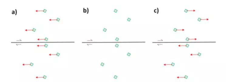
Figure 4 shows wrong answers that students tend to choose or draw. Some students think that no motion is occurring prior to an earthquake (Figure 4a), but motion must occur to build up the energy for an earthquake to occur. Other students presumably choose Figure 4b to indicate the fault is stuck, but the presence of a fault requires motion in opposite directions on opposite sides of the fault. Still other students choose Figure 4c, but equal motions on opposite sides of the fault indicate there is no friction on the fault. If an earthquake is going to occur, friction must be present to cause bending of the rocks.

The wrong answers highlight some of common misconceptions among students. When students who chose Figure 4c are told it is incorrect and why, they often indicate that they didn't realize the fault is stuck together prior to an earthquake. Students also struggle to choose Figures 3b,d as they have a hard time envisioning how the rocks are bending. This highlights limitations with this teaching approach (Table 1), including that students cannot watch the time progression when deciding on an answer, and that the approach requires students to mentally connect the map to a broad physical area. Another key issue is that most students will not have prior knowledge of GPS velocity vectors, which limits their ability to infer motion from them. GPS velocities can be reported with various frames of reference to highlight motion relative to different points of view, but the lack of interactive maps makes it difficult for students to learn this mental manipulation skill. These struggles highlight that while GPS velocity patterns are a boon to geoscientists and provide opportunities to utilize real data in the classroom, more work is needed to examine optimal strategies for using this more abstract model for elastic rebound.